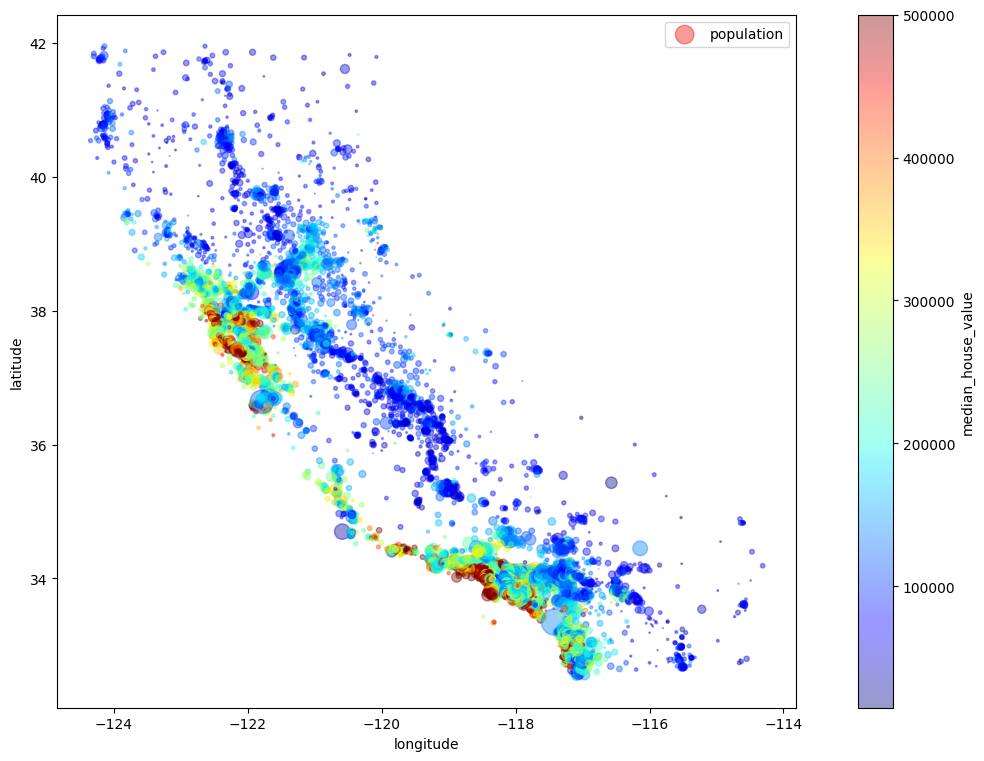
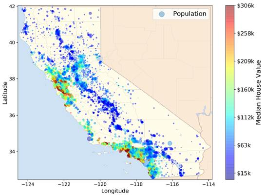
Our task is to use California census data to forecast housing prices given the population, median income, and median housing price for each block group in California. Block groups are the smallest geographical unit for which the US Census Bureau publishes sample data (a block group typically has a population of 600 to 3,000 people). We will just call them “districts” for short.
ocean_proximity is a text attribute, but not all machine libraries can manipulated textual data types.
Code
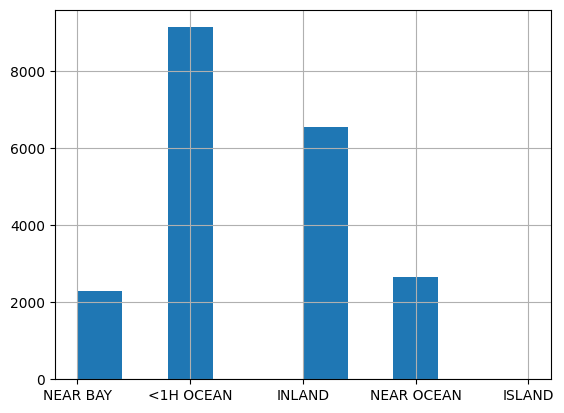
df["ocean_proximity"].value_counts()
count
ocean_proximity
<1H OCEAN
9136
INLAND
6551
NEAR OCEAN
2658
NEAR BAY
2290
ISLAND
5
Code
df["ocean_proximity"].hist()
Code
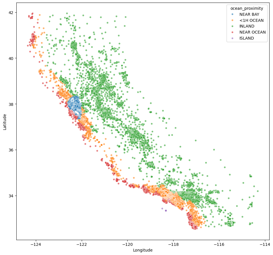
import seaborn as snsimport matplotlib.pyplot as pltplt.figure(figsize=(16, 9))sns.scatterplot(data=df, x="longitude", y="latitude", hue="ocean_proximity", alpha=0.6, s=20)plt.gca().set_aspect('equal', adjustable='box')plt.xlabel("Longitude")plt.ylabel("Latitude")plt.tight_layout()
Missing values
There are some missing values for total_bedrooms. What should we do?
Most Machine Learning algorithms cannot work with missing features.
Memory usage
What if I change float64 to float32?
Code
dff = df.copy(deep=True) # copy the dataframefor x in df.columns: # iterate over the columnsif dff[x].dtype =='float64': # if the column has type `float64` dff[x] = dff[x].astype('float32') # ... change it to `float32`dff.info() # show some statistics on the dataframe
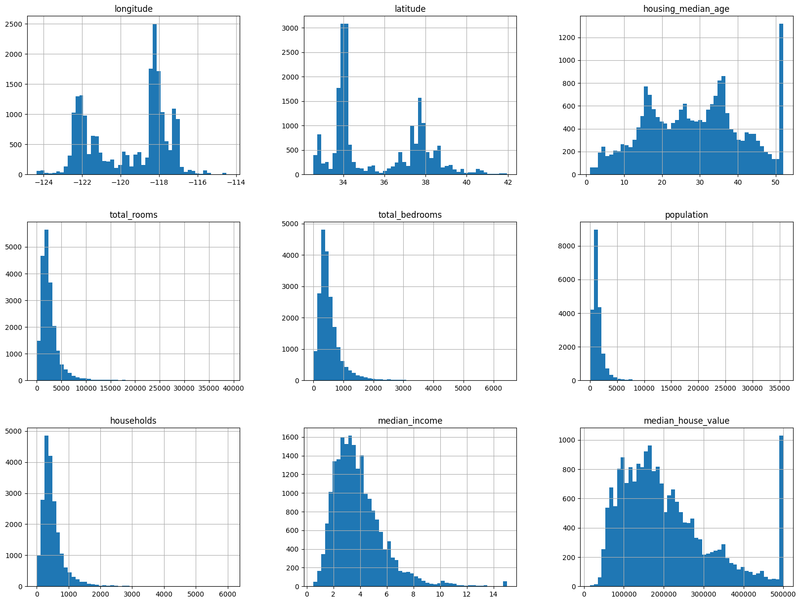
import matplotlib.pyplot as plt%matplotlib inlinedf.hist(bins=50, figsize=(20, 15))plt.show()
Open questions
median_income should be in dollars. However, it has a strange range. Why? “you are told that the data has been scaled and capped at 15 (actually 15.0001) for higher median incomes, and at 0.5 (actually 0.4999) for lower median incomes. The numbers represent roughly tens of thousands of dollars. The numbers represent roughly tens of thousands of dollars”
housing_median_age and median_house_value are capped. As to median_house_value, this is a serious problem since it is your target attribute (your labels). Your Machine Learning algorithms may learn that prices never go beyond that limit. You need to check with your client team (the team that will use your system’s output) to see if this is a problem or not. If they tell you that they need precise predictions even beyond 500,000USD, then you have mainly two options: (a) collect proper labels for the districts whose labels were capped, (b) remove those districts from the training set.”
These attributes have very different scales. Should we scale them?
Many histograms are tail heavy: they extend much farther to the right of the median than to the left. This may make it a bit harder for some Machine Learning algorithms to detect patterns
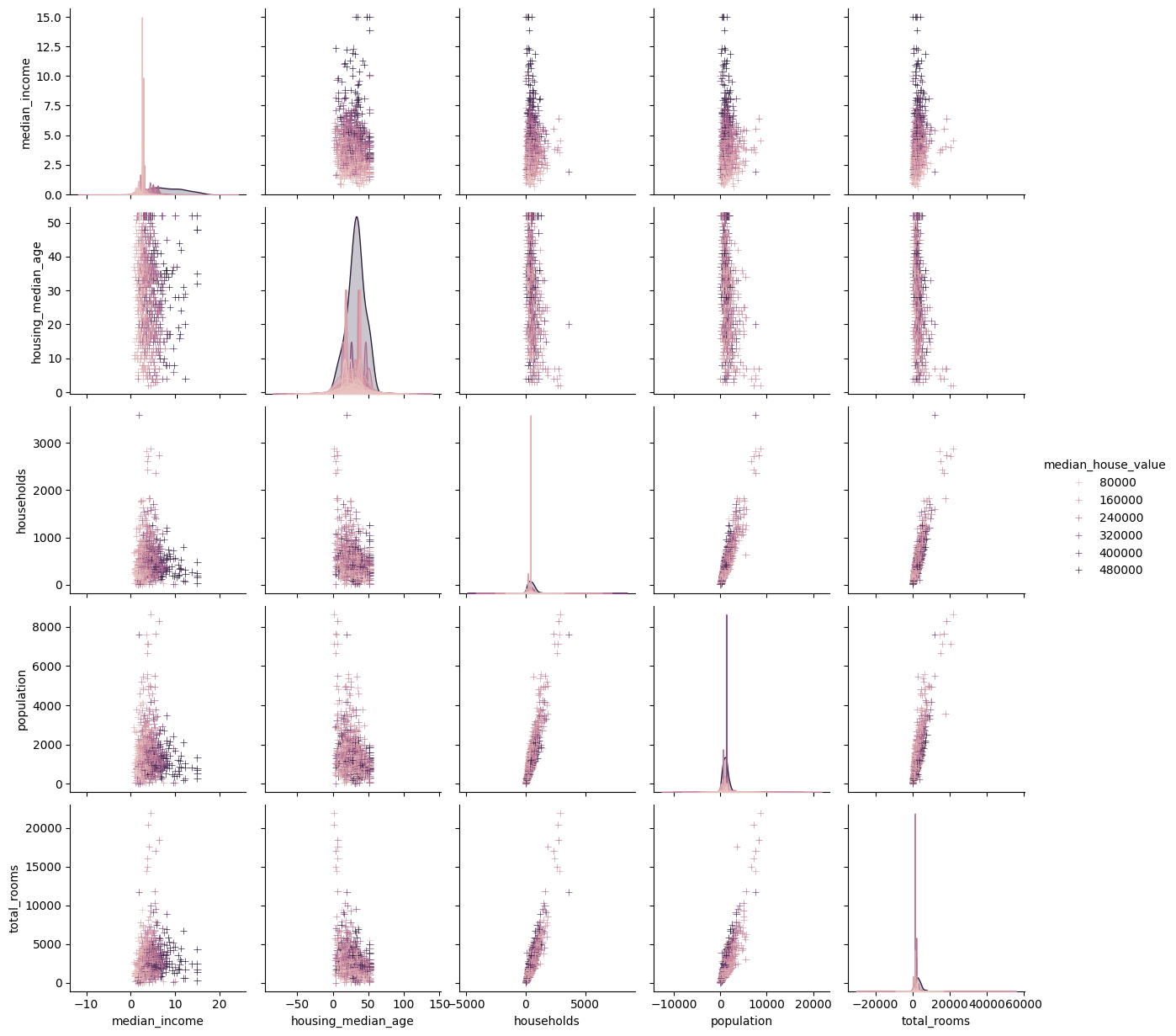
Relationships between variables
Each numeric variable in data will by shared across the y-axes across a single row and the x-axes across a single column
The diagonal plots are treated differently: univariate distribution plots show the marginal distributions of the data
The skyline operator: optimization problem that computes the Pareto optimum on tuples with multiple dimensions
Skyline comes from the view on Manhattan from the Hudson River. A building is visible if it is not dominated by a building that is taller or closer to the river (two dimensions, distance to the river minimized, height maximized).
Users want hotels for a holidays to be cheap and close to the beach. However, hotels that are close to the beach are expensive.
Formally, a tuple dominates another if it is at least as good in all dimensions and better in at least one dimension.